1. Similarities
For 2 vectors \(q\) and \(x\)
- cosine: \(cos(q,x)\)
- dot product: \(\lVert q \lVert \lVert x \lVert cos(q,x)\)
- Euclidean distance: \(\lVert q-x \lVert\)
2. Content Based Filtering
The similarity measures can be use for content based filtering. When recommending a movie to a user, the similarity score is compared between the user and the movie. It is surprising to treat movie and user with the same feature space since they are 2 different kind of entities. This is just a way to measure relevance.
We can treat each user as a separate linear regression problems by following the below steps:
- Manually give each movie a score for each feature selected (e.g. romance, action)
- For each user \(j\), learn parameter \(\theta^{(j)} \in \mathbb{R}^{n+1}\), where \(n\) is the number of features
- Predict user \(j\) as rating movie \(i\) with \((\theta^{(j)})^T x^{(i)}\)
This means that each user has their own method (represented by different linear function) of rating the movies by taking the variables \(X\) as inputs.
- \(r(i,j)=1\) if user \(j\) has rated movie \(i\), otherwise 0
- \(y^{(i,j)}=\) rating by user \(j\) (if defined)
- \(\theta^{(j)}=\) parameter vector for user \(j\)
- \(x^{(i)}=\) feature vector for movie \(i\)
- For user \(j\), movie \(i\), predicted rating: \((\theta^{(j)})^Tx^{i}\)
- \(m^{(j)}=\) number of movies rated by user \(j\)
To learn \(\theta^{(j)}\), the parameter for single user \(j\):
\(\underset{\theta^{(j)}}{\operatorname{min}} \frac{1}{2m^{(j)}} \sum\limits_{i:r(i,j)=1} \left( (\theta^{(j)})^Tx^{(i)}-y^{(i,j)} \right)^2 + \frac{\lambda}{2m^{(j)}} \sum\limits_{k=1}^n (\theta^{(j)}_k)^2\)
Gradient descent update:
for \(k=0\), \(\theta_k^{(j)}:=\theta_k^{(j)} - \alpha \frac{1}{m} \sum\limits_{i:r(i,j)=1} \left( (\theta^{(j)})^T x^{(i)} - y^{(i,j)} \right) x_k^{(i)}\)
for \(k \neq 0\), \(\theta_k^{(j)}:=\theta_k^{(j)}-\alpha \frac{1}{m} \left( \sum\limits_{i:r(i,j)=1} \left( (\theta^{(j)})^T x^{(i)} - y^{(i,j)} \right) x_k^{(i)} + \lambda \theta_k^{(j)} \right)\)
3. Collaborative Filtering
Assuming that users have given their preferences, then the problem becomes as follows.
Given \(\theta^{(1)},...,\theta^{(n_u)}\) to learn \(x^{(i)}\):
\(\underset{x^{(i)}}{\operatorname{min}} \frac{1}{2} \sum\limits_{j:r(i,j)=1} \left( (\theta^{(j)})^Tx^{(i)}-y^{(i,j)} \right)^2 + \frac{\lambda}{2} \sum\limits_{k=1}^n (x^{(i)}_k)^2\)
- One way to learn both \(\theta\) and \(x\) is to performe the estimation iteratively: random initialize \(\theta\) then learn \(x\), then learn better \(\theta\), \(\to\) converges.
To minimizing \(x^{(1)},..., x^{n_m}\) and \(\theta^{(1)},...\theta^{(n_u)}\) simultaneously:
- Given \(J(x^{(1)},...,x^{(n_m)},\theta^{(1)},...,\theta^{(n_u)}) = \frac{1}{2} \sum\limits_{(i,j):r(i,j)=1} \left( (\theta^{(j)})^Tx^{(i)}-y^{(i,j)} \right)^2 + \frac{\lambda}{2} \sum\limits_{i=1}^{n_m} \sum\limits_{k=1}^n (x^{(i)}_k)^2+ \frac{\lambda}{2} \sum\limits_{j=1}^{n_u} \sum\limits_{k=1}^n (\theta^{(j)}_k)^2\)
- \(\underset{x,\theta}{\operatorname{min}} J(x^{(1)},...,x^{(n_m)}, \theta^{(1)},...,\theta^{(n_u)})\)
Gradient descent update:
\(\theta_k^{(j)}:=\theta_k^{(j)}-\alpha \frac{1}{m} \left( \sum\limits_{i:r(i,j)=1} \left( (\theta^{(j)})^T x^{(i)} - y^{(i,j)} \right) x_k^{(i)} + \lambda x_k^{(i)} \right)\)
\(x_k^{(i)}:=x_k^{(i)}-\alpha \frac{1}{m} \left( \sum\limits_{j:r(i,j)=1} \left( (\theta^{(j)})^T x^{(i)} - y^{(i,j)} \right) \theta_k^{(j)} + \lambda \theta_k^{(j)} \right)\)
4. Matrix Factorization
When recommending a movie, the algorithm should recommend
- movies similar to the ones that user has liked in the past
- movies that similar users liked
Again, both movies and users are represented in the same embedding space.
For example, there are 4 users and 5 movies:
\[Y= \begin{bmatrix} 5 & 5 & 0 & 0 \\ 5 & \mathord{?} & \mathord{?} & 0 \\ \mathord{?} & 4 & 0 & \mathord{?} \\ 0 & 0 & 5 & 4 \\ 0 & 0 & 5 & 0 \end{bmatrix}\]
Predicted ratings: \[ \begin{bmatrix} (\theta^{(1)})^Tx^{(1)} & (\theta^{(2)})^Tx^{(1)} & (\theta^{(3)})^Tx^{(1)} & (\theta^{(4)})^Tx^{(1)} \\ (\theta^{(1)})^Tx^{(2)} & (\theta^{(2)})^Tx^{(2)} & (\theta^{(3)})^Tx^{(2)} & (\theta^{(4)})^Tx^{(2)} \\ (\theta^{(1)})^Tx^{(3)} & (\theta^{(2)})^Tx^{(3)} & (\theta^{(3)})^Tx^{(3)} & (\theta^{(4)})^Tx^{(3)} \\ (\theta^{(1)})^Tx^{(4)} & (\theta^{(2)})^Tx^{(4)} & (\theta^{(3)})^Tx^{(4)} & (\theta^{(4)})^Tx^{(4)} \\ (\theta^{(1)})^Tx^{(5)} & (\theta^{(2)})^Tx^{(5)} & (\theta^{(3)})^Tx^{(5)} & (\theta^{(4)})^Tx^{(5)} \end{bmatrix} = \begin{bmatrix} (x^{(1)})\\ (x^{(2)})\\ (x^{(3)})\\ (x^{(4)})\\ (x^{(5)}) \end{bmatrix} \begin{bmatrix} \theta^{(1)} & \theta^{(2)} & \theta^{(3)} & \theta^{(4)} \end{bmatrix}= \begin{bmatrix} (x^{(1)})\\ (x^{(2)})\\ (x^{(3)})\\ (x^{(4)})\\ (x^{(5)}) \end{bmatrix} \begin{bmatrix} (\theta^{(1)})\\ (\theta^{(2)})\\ (\theta^{(3)})\\ (\theta^{(4)}) \end{bmatrix}^T = X \theta^T \]
To make the notation simplier to read:
- \(X\): item embedding \(V \in \mathbb{R}^{n_m {\times} k}\)
- \(\theta\): user embedding \(U \in \mathbb{R}^{n_u {\times} k}\)
The goal is to factorize the feedback matrix \(Y\) into the product of a user embedding matrix \(U\) (or \(\theta\) in the previous section) and item (movie) embedding matrix \(V\) (or \(X\) in the previous section) such that \(Y \approx VU^T\)
Matrix factorization, \(VU^T\) is a simple embedding model
\(\to\) cold-start problem
5. Mean Normalization
Assuming user 5 has not yet rated any movies.
\[Y= \begin{bmatrix} 5 & 5 & 0 & 0 & \mathord{?} \\ 5 & \mathord{?} & \mathord{?} & 0 & \mathord{?}\\ \mathord{?} & 4 & 0 & \mathord{?} & \mathord{?}\\ 0 & 0 & 5 & 4 & \mathord{?}\\ 0 & 0 & 5 & 0 & \mathord{?} \end{bmatrix}\]
Then, \(\theta^{(5)}\) is going to a vector of 0, as
- it is optimized only by the regularization term \(\sum\limits_{j=1}^{n_u} \sum\limits_{k=1}^n (\theta^{(j)}_k)^2\).
- The term \(\frac{1}{2} \sum\limits_{(i,j):r(i,j)=1} \left( (\theta^{(j)})^Tx^{(i)}-y^{(i,j)} \right)^2\) does not affect \(\theta^{(5)}\) as \(r(i,j)=0\) for \(i=5\)
The resulting predicted ratings for all movies rated by user 5 would then be 0 given by \((\theta^{(5)})^Tx^{(i)} = 0\) which is not very useful.
Solution- mean normalization (mean for \((i,j)\) where \(r(i,j)=1\)). The mean vector \(mu\) of the feedback matrix \(Y\) is:
\[ \mu = \begin{bmatrix} 2.5\\ 2.5\\ 2\\ 2.25\\ 1.25 \end{bmatrix} \]
Then, the mean normalized feedback matrix \(Y\) becomes: \[Y= \begin{bmatrix} 2.5 & 2.5 & -2.5 & -2.5 & \mathord{?} \\ 2.5 & \mathord{?} & \mathord{?} & -2.5 & \mathord{?}\\ \mathord{?} & 2 & -2 & \mathord{?} & \mathord{?}\\ -2.25 & -2.25 & 2.75 & 1.75 & \mathord{?}\\ -1.25 & -1.25 & 3.75 & -1.25 & \mathord{?} \end{bmatrix}\]
Then learn \(\theta^{(j)}\) and \(x^{(i)}\) using the mean normalized feedback matrix. The prediction for user \(j\) and movie \(i\) would be:
\[(\theta^{(j)})^Tx^{(i)} + \mu_i\]
The intuition is that if the user hasn’t rated any movies, the the prediction for movie \(i\) is just going to be the average rating of movie \(i\).
On the other hand, if there is a movie that hasn’t been rated by any user, the mean normalization can be applied to column.
6. Choose the Loss Function
The below loss function comparison are shown without regularization terms:
- Observing only: only sum over observed pairs \[J(x^{(1)},...,x^{(n_m)},\theta^{(1)},...,\theta^{(n_u)}) = \frac{1}{2} \sum\limits_{(i,j):r(i,j)=1} \left( (\theta^{(j)})^Tx^{(i)}-y^{(i,j)} \right)^2\]
- treat the unobserved values \(y^{(i,j)}\) as zero: Singular Value Decomposition (SVD) \[J(x^{(1)},...,x^{(n_m)},\theta^{(1)},...,\theta^{(n_u)}) = \frac{1}{2} \sum\limits_{(i,j)} \left( (\theta^{(j)})^Tx^{(i)}-y^{(i,j)} \right)^2\]
- Weighted Matrix Factorization - decomposes the objective into the following two sums:
- A sum over observed entries.
- A sum over unobserved entries (treated as zeroes). \[J(x^{(1)},...,x^{(n_m)},\theta^{(1)},...,\theta^{(n_u)}) = \frac{1}{2} \sum\limits_{(i,j):r(i,j)=1} w_{i,j} \left( (\theta^{(j)})^Tx^{(i)}-y^{(i,j)} \right)^2 + \frac{1}{2} \sum\limits_{(i,j):r(i,j)=0} w_{0}\left( (\theta^{(j)})^Tx^{(i)} \right)^2\] where \(w_{i,j}\)is a function of the frequency of movie \(i\) and user \(j\), “\(w_0\) is a hyperparameter that weights the two terms so that the objective is not dominated by one or the other. Tuning this hyperparameter is very important.”
7. Stochastic Gradient Descent
The (batch) gradient descent approach becomes computational expensive when the data is large.
- Randomly shuffle dataset
Another approach called Mini-batch Gradient Descent lies somewhere between the (batch) gradient and stochastic gradient descent.
8. Weighted Alternating LS
Weighted Alternating Least Squares (WALS)
9. Example: MovieLens Data
## Warning in doTryCatch(return(expr), name, parentenv, handler): unable to load shared object '/Library/Frameworks/R.framework/Resources/modules//R_X11.so':
##   dlopen(/Library/Frameworks/R.framework/Resources/modules//R_X11.so, 6): Library not loaded: /opt/X11/lib/libSM.6.dylib
##   Referenced from: /Library/Frameworks/R.framework/Versions/3.5/Resources/modules/R_X11.so
##   Reason: image not found
# load data
user <- read.csv("/Users/smartboyben/Documents/Data/MovieLens/u.user",sep="|",header=FALSE)
colnames(user) <- c('user_id', 'age', 'sex', 'occupation', 'zip_code')
ratings <- read.csv('/Users/smartboyben/Documents/Data/MovieLens/u.data',sep='\t')
colnames(ratings) <- c('user_id', 'movie_id', 'rating', 'unix_timestamp')
movies <- read.csv('/Users/smartboyben/Documents/Data/MovieLens/u.item',sep="|",header=FALSE)
# The movies file contains a binary feature for each genre.
genre_cols <- c(
"genre_unknown", "Action", "Adventure", "Animation", "Children", "Comedy",
"Crime", "Documentary", "Drama", "Fantasy", "Film-Noir", "Horror",
"Musical", "Mystery", "Romance", "Sci-Fi", "Thriller", "War", "Western"
)
colnames(movies) <- c('movie_id', 'title', 'release_date', "video_release_date", "imdb_url",genre_cols)
colnames(movies)[[16]] <- "Film_Noir"
colnames(movies)[[21]] <- "Sci_Fi"
rating_DF <- full_join(
x=ratings,
y=user,
by = ("user_id"="user_id"),
copy = FALSE,
suffix = c(".rating", ".user"),
keep = FALSE
)
rating_DF <- full_join(
x=rating_DF,
y=movies,
by = ("movie_id"="movie_id"),
copy = FALSE,
suffix = c(".rating", ".movie"),
keep = FALSE
)9.1 Data Exploration
In this dataset, the number of users, 943, is less than the number of movies, 1,682. In reality though, there should be a lot more user than movies.
cat("unique users:",nrow(user),"\n")## unique users: 943cat("unique movies:",nrow(movies))## unique movies: 1682user_rating_avg <- sqldf("
select user_id
, count(*) as rate_number
, avg(rating) as avg_user_rating
from rating_DF
group by 1
", drv="SQLite")
par(mfrow=c(1,2))
hist(user_rating_avg[,"avg_user_rating"], xlab='rating',main="Users' Average Rating", breaks = 20)
hist(user_rating_avg[,"rate_number"], xlab='Number of movies that a user has rated',main="Number of movies that a user has rated", breaks = 150, xlim=c(0,150))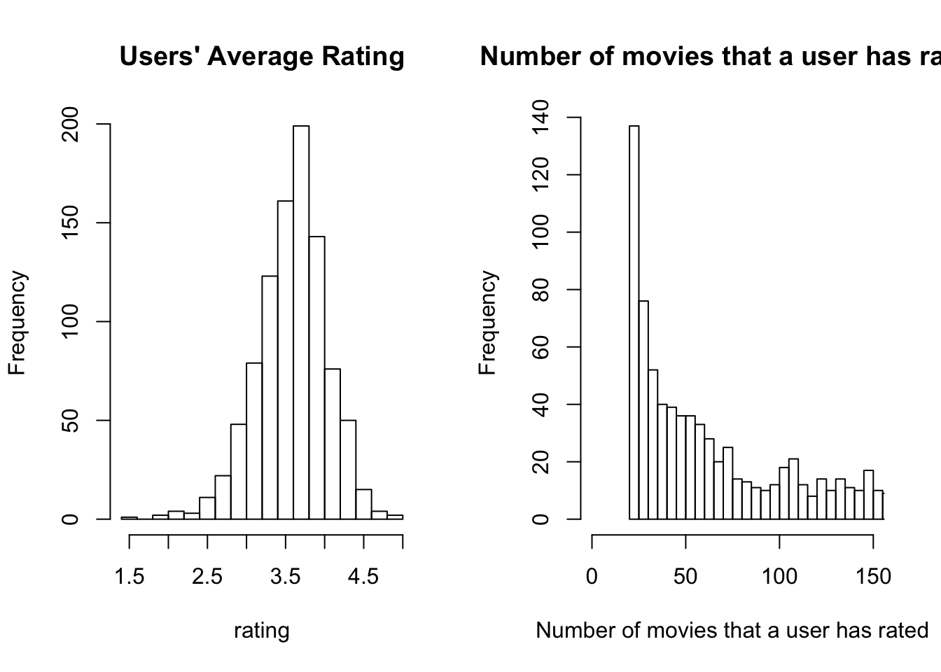
movie_rating_avg <- sqldf("
select movie_id
, count(*) as rated_count
, avg(rating) as avg_movie_rating
from rating_DF
group by 1
", drv="SQLite")

par(mfrow=c(1,2))
hist(movie_rating_avg[which(movie_rating_avg$rated_count>10),"avg_movie_rating"], xlab='rating',main="Movies' Average Rating", breaks=20)
hist(movie_rating_avg[,"rated_count"], xlab='Number of times a movies is rated',main="Number of times a movies is rated", breaks=300, xlim=c(0,30))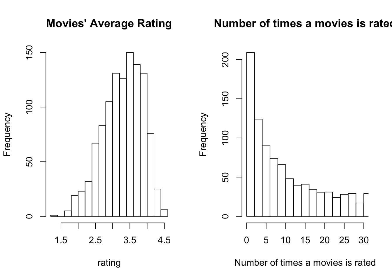
## contruct feedback matrix
ratings <- sqldf("
select * from ratings order by movie_id, user_id asc
                 ",drv="SQLite")

Y_feedback <- reshape(ratings[,c("movie_id","user_id","rating")], idvar = "movie_id", timevar = "user_id", direction = "wide",sep="_")
rownames(Y_feedback) <- Y_feedback$movie_id
Y_feedback$movie_id <- NULL
Y <- Y_feedback

## movie vectors
V <- movies[,c(6:ncol(movies))]
rownames(V) <- movies$movie_id
V <- as.matrix(V)
## user vectors
U <- data.frame(matrix(NA, nrow=nrow(user), ncol=ncol(V)))
rownames(U) <- user$user_id
GD_optimize_U <- function(Y, U, V, learning_rate=10, regularization=TRUE, lambda=1) {
## initialize the parameters for V
initial_U <- sample(c(0,1), replace=TRUE, size=(nrow(U)*ncol(U)))
initial_U <- matrix(initial_U, nrow=nrow(U), ncol=ncol(U))
U <- initial_U
approx_Y <- V%*%t(U)
m <- length(which(!is.na(Y)))
r <- which(!is.na(Y),arr.ind=TRUE)
for(i in 1:1000) {
if(regularization==TRUE) {
U <- U - learning_rate * ( (Y[r[i,1],r[i,2]]-approx_Y[r[i,1],r[i,2]])*V[i,] + lambda*U )
approx_Y <- V%*%t(U)
#loss <- 1/(2*m)*sum(Y-approx_Y)
#loss <- loss + sum(U^2)/(2*m) + sum(V^2)/(2*m)
} else {
temp <- sum(Y-approx_Y,na.rm = TRUE) *V
U <- U - learning_rate * temp/m
approx_Y <- V%*%t(U)
#loss <- 1/(2*m)*sum(Y-approx_Y)
}
}
return(U)
}9.2 SGD without Regularization
SGD_optimize_U <- function(Y, U, V, learning_rate=10, iterations=10, regularization=TRUE, lambda=1) {
  ## initialize the parameters for V
  initial_U <- sample(c(0,1), replace=TRUE, size=(nrow(U)*ncol(U)))
  initial_U <- matrix(initial_U, nrow=nrow(U), ncol=ncol(U))
  U <- initial_U
  approx_Y <- V%*%t(U)
  m <- length(which(!is.na(Y)))
  # loss <- 1/(2*m)*sum(Y-approx_Y)
  # if(regularization==TRUE) {
  #   loss <- loss + sum(U^2)/(2*m) + sum(V^2)/(2*m)
  # }
  r <- which(!is.na(Y),arr.ind=TRUE)
  for(i in 1:m) {
    if(regularization==TRUE) {
      U <- U - learning_rate * ( (Y[r[i,1],r[i,2]]-approx_Y[r[i,1],r[i,2]])*V[i,] + lambda*U )
      approx_Y <- V%*%t(U)
      #loss <- 1/(2*m)*sum(Y-approx_Y)
      #loss <- loss + sum(U^2)/(2*m) + sum(V^2)/(2*m)
    } else {
      temp <- ( Y[r[i,1],r[i,2]]-approx_Y[r[i,1],r[i,2]] ) *V[r[i,1],]
      temp <- do.call("rbind", replicate(nrow(U), temp, simplify = FALSE))
      U <- U - learning_rate * temp
      approx_Y <- V%*%t(U)
      #loss <- 1/(2*m)*sum(Y-approx_Y)
    }
  }
  return(U)
}

#test <- SGD_optimize_U(Y, U, V, regularization = FALSE)
#nonRegularized_U <- SGD_optimize_U(Y=Y_feedback, U=U, V=V, learning_rate = 0.001, regularization=FALSE)