Logistic Regression & Information Value (IV)
Introduction
To solve a classification problem, \(y_i\) is either \(0\) or \(1\), we want to estimate the probability of \(y_i=1\) by a set of explanatory variable \(X\), denoted as \(p(x)\). However, we cannot simply model the probability by the linear regression model as \(p(x) = \beta_0 + x \beta\) since the probability is bound between [0,1] whereas the linear function of the explanatory variables is unbounded.
By transforming the probability to log odds ratio, the target variable becomes unbounded and can be expressed as iinear function of the explanatory variables: \[log\frac{p(x)}{1-p(x)} = \beta_0 + x\beta\] Now the equation looks like an OLS. When transforming the data to log(odds), the target variable becomes positive and negative infinity, and therefore the residuals cannot be calculated. To estimate the \(\beta\)s, we can use the maximum likelihood or gradient descent.
The probability can be expressed as the log(odds): \[ \begin{aligned} log(\frac{p}{1-p}) &= log(odds) \\ \frac{p}{1-p} &= e^{log(odds)} \\ p &= (1-p)e^{log(odds)} \\ p &= e^{log(odds)}-pe^{log(odds)} \\ p+pe^{log(odds)} &=e^{log(odds)}\\ p &= \frac{e^{log(odds)}}{1+e^{log(odds)}} \end{aligned} \]
To estimate the probability directly, we define the probability estimator as:
\[\hat p = h_{\theta}(x) = \sigma(\beta_0+x\beta)\]
where \(\sigma\) is the sigmoid function \(\sigma(t) = \frac{1}{1+e^{-t}}\)
t <- seq(-10,10, length=40)
sigmoid_t <- 1/(1+exp(-t))
plot(t, sigmoid_t, col="blue", lwd=2,type='l')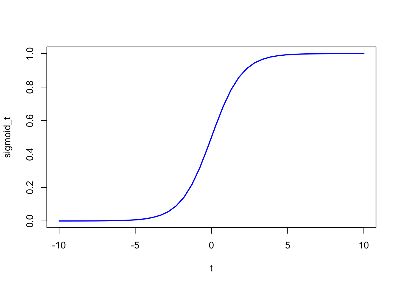
\(\hat y = 0 \,\, if \,\,\hat p<0.5\) and \(\hat y = 1 \,\, if \,\,\hat p\geq0.5\)
or more explicitly,
\[\hat p = \frac{1}{1+e^{-(\beta_0+x\beta)}}\]
Cost Function
singel training instance cost function: \[ c(\beta_0, \beta) = \begin{cases} -log(\hat p) & \quad \text{if } y=1\\ -log(1-\hat p) & \quad \text{if } y=0 \end{cases} \] logistic regression cost function: \[l(\beta_0, \beta) = -\frac{1}{n}\sum_{i=1}^{n}[y_ilog(\hat p)+(1-y_i)log(1-\hat p)]\] It’s similar to the log likelihood function, where we can define the likelihood function as the equation below, assuming the likelihood of obvervations are independent of each other given explanatory variables \(X\):
\[ L(\beta_0, \beta) = \prod_{i=1}^{n}p(x_i)^{y_i}(1-p(x_i)^{1-y_i})\] then log-likelihood function is:
\[l(\beta_0, \beta) = \sum_{i=1}^{n}y_i(log(p(x_i)))+(1-y_i)log(1-p(x_i)) \]
The estimation can either done by minimize the cost function or maximize the log-likelihood function
logistic cost function partial derivatives: \[\frac{\partial}{\partial \theta_j}l(\theta) = \frac{1}{n}\sum_{i=1}^{n}(\sigma(\theta^T x^{(i)}-y^{(i)}))x_j^{(i)}\] The logistic regression does not have analytical solution, it must be solved numerically.
Goodness of Fit
We discuss one of the ways to measure the goodness of fit.
McFadden’s psuedo \(R^2\)
Recall that the \(R^2=\frac{SS(mean)-SS(fit)}{SS(mean)}\) in linear regression where \(SS\) means the sum of residual’s square \(SS(mean)\) is the sum of residual’s square where the prediction is just the average of the sample target variable. However, we can’t use the residual.
We use \(LL(fit)\) for the log-likelihood of the fitted line, and use it as a substitute for \(SS(fit)\). Now we need to substitution for \(SS(mean)\). For benchmarking purpose, we have to find substitution for \(SS(mean)\). We can use the log-likelihood of the estimation with no explanatory variable. This would be the log-likelihood with the estimate of probability \(\hat{p}\) equals to the sum of \(y\) divided by number of observations. We denote this as \(LL(0)\). Now we have the McFadden’s psuedo \[R^2 = \frac{LL(0)-LL(fit)}{LL(0)}\]
We use the null and saturated model to calculate the proposed model’s R square and p-value
- Null model: an oversimplified model
- Saturated model: an over-complicated model
Review R squuare for linear regression: \[R^2 = \frac{SS(Null\ Model)-SS(Proposed\ Model)}{SS(Null\ Model)}\] Null Model here is the average of the target variable.
Now for log-likelihood based R square:
\[R^2 = \frac{LL(Null \ Model)-LL(Proposed \ Model)}{LL(Null \ Model)-LL(Saturated \ Model)}\]
The inclusion of saturated model ensures that the R square is between 0 and 1!
- Residual deviance: \(2 \cdot (LL(Saturated \ Model)-LL(Proposed \ Model))\) follows Chi-square distribution. For this to work, the proposed model has to be a simpler version of the saturated model
- Null deviance: \(2 \cdot (LL(Saturated \ Model)-LL(Null \ Model))\)
- \(Null Deviance - Residual Deviance\) is a Chi-square value with degree of freedom equal to the difference in the number of parameters for the proposed Model and the Null Model
- Deviance residuals: \(\sum_i^N \sqrt{2 \cdot LL(Saturated \ Model)_i - LL(ProposedModel)_i}\), it is Analogous to the residuals of OLS.
Logistic regression is a special case where we can ingnore the saturated model when calculating the R swuare as the \(LL(Saturated \ Model)=0\).
The glm function in R for logistic regression returns residual deviance and null deviance which can be used for calculating the McFadden’s psuedo \(R^2\)
Wald Statistics The wald test in logistic regression is the test analogic to the t-test for coefficients in linear regression.
\[w = (\hat{\theta}-\hat{\theta}_0)^{T}[Var(\hat{\theta})]^{-1}(\hat{\theta}-\hat{\theta}_0)\]
To better illustrate the intuition, we assume \(\hat{\theta}\) is one-dimensional, then under the Null hypothesis:
\[w = \frac{(\hat{\theta}-\theta_0)^2}{Var(\hat{\theta})} \sim \chi_1^2\]
Information Value (IV) and WOE
Information Value (IV) and Weight of Evidence (WOE)
Weight of evidence (WOE): \[WOE = ln(\frac{\% \ of \ non-event}{\% \ of \ event})\]
Steps:
- For continuous variable, split the data into n bucket. If the variable is categorical , nothing needs to be done for this step.
- Apply the formula above for each bucket.
- Note that WOE is usually positive as non-event is usually less than event.
- The greater the value of WOE, the higher the chance of observing Y=1.
Information Value (IV):
\[IV = \sum_{i=1}^n \ (\% \ of \ NonEvent - \% \ of \ Event) \cdot WOE\] The IV is commonly used for variable selection & univariate analysis for logistic regression as the logic is similar to log-odds ratio which is used in logistic regression. Variable selection using IV will not be optimal for classification algorithm other than logistic regression.