Predicting Churns
The purpose of this section is to use tree-based algorithm to predict churn of a customr based on some explanatory variable. The data I use is the Customer Support data from IBM Watson Analytics.
library(survival)
library(ggfortify)
library(rpart)
library(dplyr)
churnAnalysis <- read.csv("WA_Fn-UseC_-Telco-Customer-Churn.csv")
churnAnalysis <- as.data.frame(churnAnalysis)
#head(churnAnalysis)
1. Data pre-processing
Check if there is missing value. There are only 11 missing values in TotalCharges so we can just remove entire row given that the number is small.
sapply(churnAnalysis, function(x) sum(is.na(x)))## customerID gender SeniorCitizen Partner
## 0 0 0 0
## Dependents tenure PhoneService MultipleLines
## 0 0 0 0
## InternetService OnlineSecurity OnlineBackup DeviceProtection
## 0 0 0 0
## TechSupport StreamingTV StreamingMovies Contract
## 0 0 0 0
## PaperlessBilling PaymentMethod MonthlyCharges TotalCharges
## 0 0 0 11
## Churn
## 0churnAnalysis <- churnAnalysis[which(!is.na(churnAnalysis[,"TotalCharges"])),]Then we look at what variables are continuous, and they are: “tenure”, “MonthlyCharges” and “TotalCharges”
2. Kaplan Meier Analysis
library(survival)
library(ggfortify)
churnAnalysis <- churnAnalysis %>% mutate(Churn_flag = ifelse(Churn=="Yes", 1, 0) )
km_churn <- with(churnAnalysis, Surv(tenure, Churn_flag))
km_fit <- survfit(Surv(tenure, Churn_flag) ~ 1, data=churnAnalysis)
autoplot(km_fit)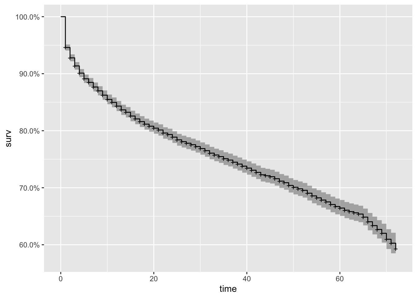
The figure below shows the conditional churn probability given that the account “survived” the last period. We can see that the churn rate is the highest in the first time unit and gradually reverts to the mean at around 10th time unit.
# Conditional churn probability
s0 <- c(1,km_fit$surv[1:71])
c <- (1-km_fit$surv)/s0
c <- (s0-km_fit$surv)/s0
plot(c, type='l')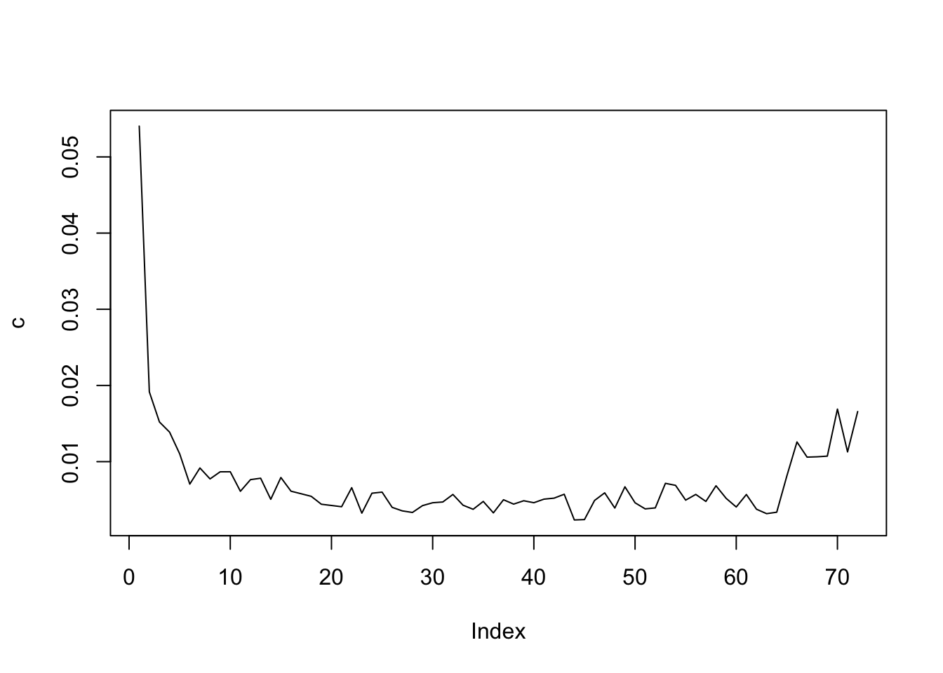
km_fit_bill <- survfit(Surv(tenure, Churn_flag) ~ PaperlessBilling, data=churnAnalysis)
autoplot(km_fit_bill)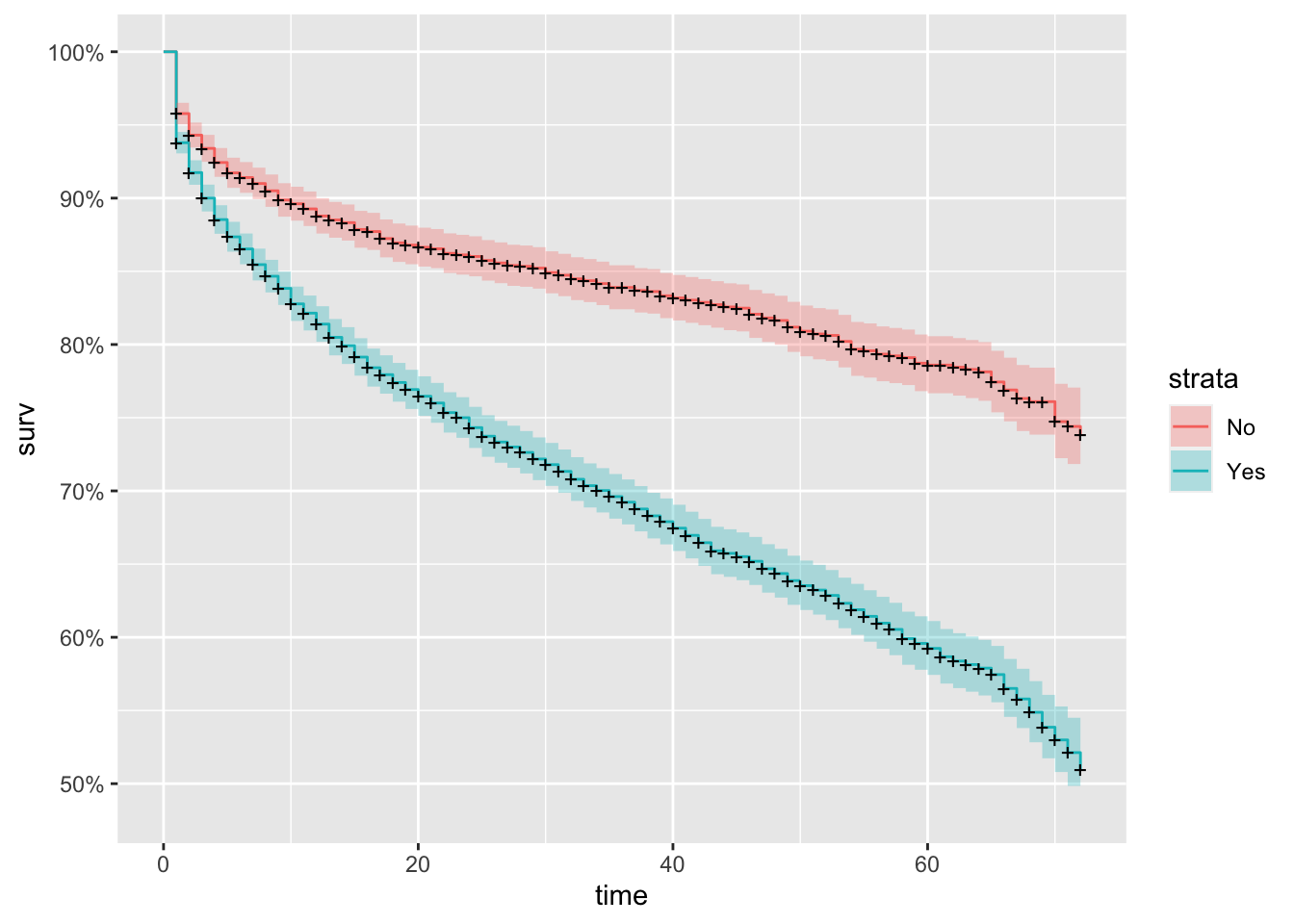
km_fit_senior <- survfit(Surv(tenure, Churn_flag) ~ SeniorCitizen, data=churnAnalysis)
autoplot(km_fit_senior)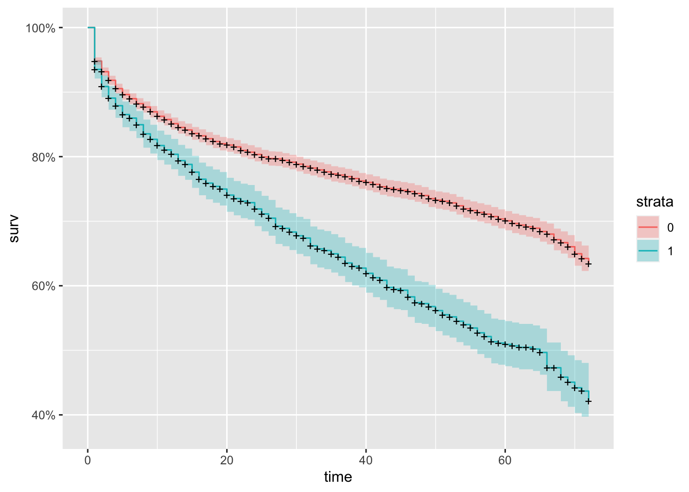
km_fit_pay <- survfit(Surv(tenure, Churn_flag) ~ PaymentMethod, data=churnAnalysis)
autoplot(km_fit_pay)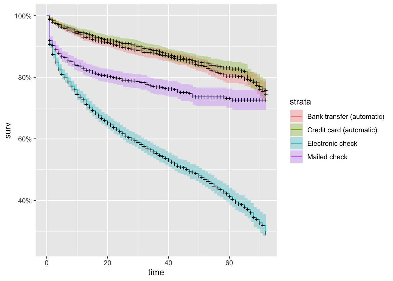
3. Information value
##
## Attaching package: 'kableExtra'
## The following object is masked from 'package:dplyr':
##
## group_rows| Variable | IV |
|---|---|
| Contract | 1.2331890 |
| tenure | 0.8347032 |
| OnlineSecurity | 0.7152919 |
| TechSupport | 0.6971084 |
| InternetService | 0.6152530 |
| OnlineBackup | 0.5264879 |
| DeviceProtection | 0.4976099 |
| PaymentMethod | 0.4557558 |
| StreamingMovies | 0.3798511 |
| StreamingTV | 0.3787158 |
| Variable | IV | |
|---|---|---|
| 11 | MonthlyCharges | 0.3631453 |
| 12 | TotalCharges | 0.3376950 |
| 13 | PaperlessBilling | 0.2020563 |
| 14 | Dependents | 0.1531686 |
| 15 | Partner | 0.1178772 |
| 16 | SeniorCitizen | 0.1050842 |
| 17 | MultipleLines | 0.0081689 |
| 18 | PhoneService | 0.0007129 |
| 19 | gender | 0.0003741 |
| NA | NA | NA |
4. logistic regression with WOEs
Under contruction
5. Decision tree by rpart
To use decision tree, we need to convert the continuous variables to categorical variables be setting some thresold. But first, let’s split the data into training, validation and test sets.
## randomize the data first
churnAnalysis <- churnAnalysis[sample(1:nrow(churnAnalysis)),]
## then split
churnAnalysisTraining <- churnAnalysis[1:(nrow(churnAnalysis)/2),]
churnAnalysisValidation <- churnAnalysis[(nrow(churnAnalysis)/2+1): (3*nrow(churnAnalysis)/4),]
churnAnalysisTest <- churnAnalysis[(3*nrow(churnAnalysis)/4+1),nrow(churnAnalysis),]
hist(churnAnalysisTraining[,"MonthlyCharges"],breaks=40)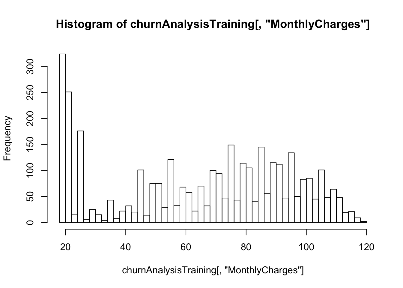
MonthlyChargesClass <- ifelse(churnAnalysis[,"MonthlyCharges"]<=30,"<=$30",">30$")As the distribtion of “MonthlyCharges” does look like normal distribution and there seems to be a spike for monthly charges under 30. Hence, I try to split the data into 2:
1. monthly charges $ 30 $
2. monthly charges $ > 30 $
hist(churnAnalysisTraining[,"TotalCharges"],breaks=40)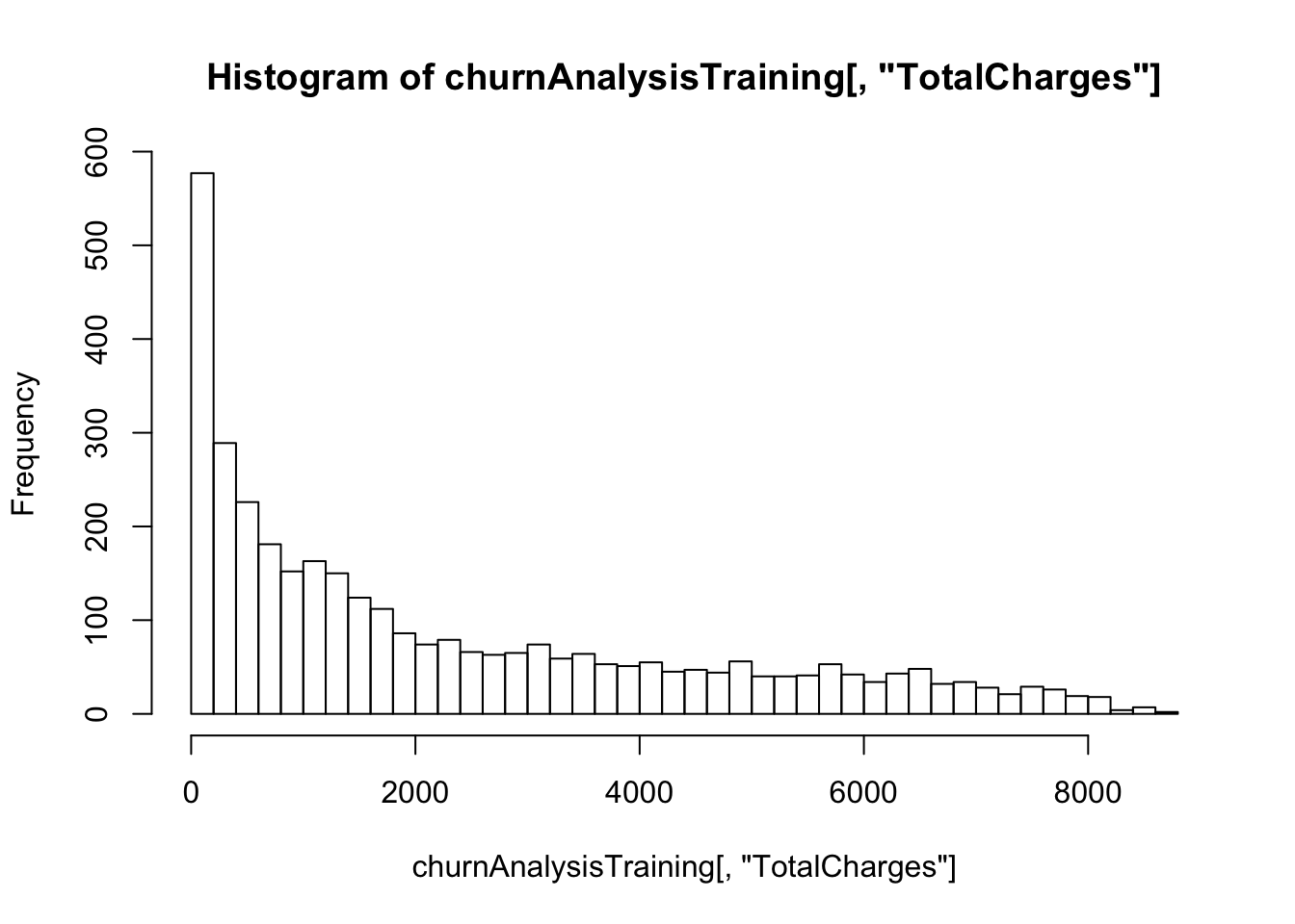
TotalChargesClass <- ifelse(churnAnalysis[,"TotalCharges"]<=500,"<=$500",">500$")hist(churnAnalysisTraining[,"tenure"],breaks=80)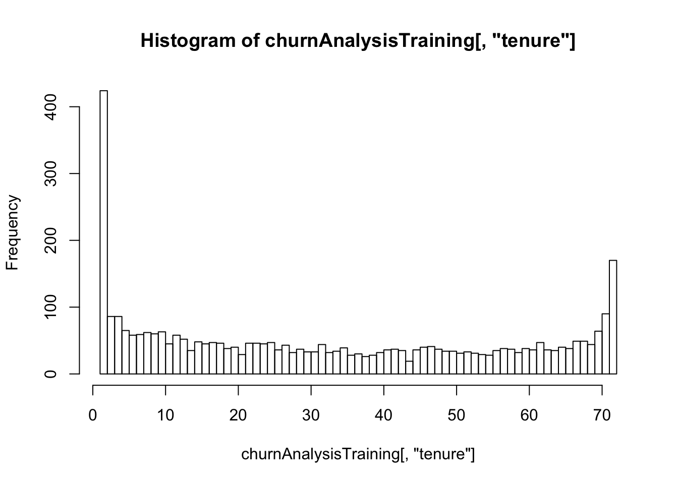
TenureClass <- churnAnalysis[,"tenure"]
TenureClass[which(churnAnalysis[,"tenure"] >=70)] <- ">=70"
TenureClass[which(churnAnalysis[,"tenure"] <=5)] <- "<=5"
TenureClass[which(churnAnalysis[,"tenure"] >5 & churnAnalysis[,"tenure"] <70)] <- "between"
Apply the class transform to all 3 data sets
churnAnalysis["MonthlyCharges"] <- MonthlyChargesClass
churnAnalysis["TotalCharges"] <- TotalChargesClass
churnAnalysis["tenure"] <- TenureClass
churnAnalysisTraining <- churnAnalysis[1:(nrow(churnAnalysis)/2),]
churnAnalysisValidation <- churnAnalysis[(nrow(churnAnalysis)/2+1): floor(3*nrow(churnAnalysis)/4),]
churnAnalysisTest <- churnAnalysis[floor(3*nrow(churnAnalysis)/4+1):nrow(churnAnalysis),]
use rpart to run decision tree from package:rpart
library(rpart)
## xval determine how many data points you want in the validation set.
fitTree <- rpart(Churn~gender+SeniorCitizen+Partner+Dependents+tenure+PhoneService+MultipleLines+InternetService+OnlineSecurity+OnlineBackup+DeviceProtection+TechSupport+StreamingTV+StreamingMovies+Contract+PaperlessBilling+PaymentMethod+MonthlyCharges+TotalCharges, churnAnalysisTraining,xval=0)
pred_fitTree <- predict(fitTree, churnAnalysisTest,type="class")
table(Predicted = pred_fitTree, Actual = churnAnalysisTest$Churn) ## Confusion Matrix for Decision Tree
## Actual
## Predicted No Yes
## No 1193 290
## Yes 108 167plot(fitTree,uniform=TRUE)
text(fitTree,use.n=T,all=T)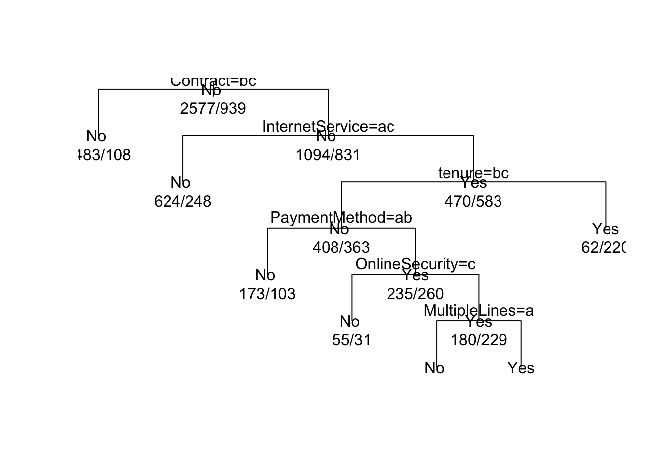
printcp(fitTree) ## cp : complexity parameter##
## Classification tree:
## rpart(formula = Churn ~ gender + SeniorCitizen + Partner + Dependents +
## tenure + PhoneService + MultipleLines + InternetService +
## OnlineSecurity + OnlineBackup + DeviceProtection + TechSupport +
## StreamingTV + StreamingMovies + Contract + PaperlessBilling +
## PaymentMethod + MonthlyCharges + TotalCharges, data = churnAnalysisTraining,
## xval = 0)
##
## Variables actually used in tree construction:
## [1] Contract InternetService MultipleLines OnlineSecurity
## [5] PaymentMethod tenure
##
## Root node error: 939/3516 = 0.26706
##
## n= 3516
##
## CP nsplit rel error
## 1 0.060170 0 1.00000
## 2 0.047923 2 0.87966
## 3 0.026624 3 0.83174
## 4 0.025559 4 0.80511
## 5 0.013845 5 0.77955
## 6 0.010000 6 0.76571The cp at row one is the (rel error at row 2 - rel error at row 1)/nsplit in row 2. The “rel error” is the relative error = absolute error/root node error
now prune the tree using the validation set
TreeDepth <- nrow(fitTree$cptable)
for(i in 2:TreeDepth)
printcp(fitTree)##
## Classification tree:
## rpart(formula = Churn ~ gender + SeniorCitizen + Partner + Dependents +
## tenure + PhoneService + MultipleLines + InternetService +
## OnlineSecurity + OnlineBackup + DeviceProtection + TechSupport +
## StreamingTV + StreamingMovies + Contract + PaperlessBilling +
## PaymentMethod + MonthlyCharges + TotalCharges, data = churnAnalysisTraining,
## xval = 0)
##
## Variables actually used in tree construction:
## [1] Contract InternetService MultipleLines OnlineSecurity
## [5] PaymentMethod tenure
##
## Root node error: 939/3516 = 0.26706
##
## n= 3516
##
## CP nsplit rel error
## 1 0.060170 0 1.00000
## 2 0.047923 2 0.87966
## 3 0.026624 3 0.83174
## 4 0.025559 4 0.80511
## 5 0.013845 5 0.77955
## 6 0.010000 6 0.76571
##
## Classification tree:
## rpart(formula = Churn ~ gender + SeniorCitizen + Partner + Dependents +
##     tenure + PhoneService + MultipleLines + InternetService +
##     OnlineSecurity + OnlineBackup + DeviceProtection + TechSupport +
##     StreamingTV + StreamingMovies + Contract + PaperlessBilling +
##     PaymentMethod + MonthlyCharges + TotalCharges, data = churnAnalysisTraining,
##     xval = 0)
##
## Variables actually used in tree construction:
## [1] Contract        InternetService MultipleLines   OnlineSecurity
## [5] PaymentMethod   tenure
##
## Root node error: 939/3516 = 0.26706
##
## n= 3516
##
##         CP nsplit rel error
## 1 0.060170      0   1.00000
## 2 0.047923      2   0.87966
## 3 0.026624      3   0.83174
## 4 0.025559      4   0.80511
## 5 0.013845      5   0.77955
## 6 0.010000      6   0.76571
##
## Classification tree:
## rpart(formula = Churn ~ gender + SeniorCitizen + Partner + Dependents +
## tenure + PhoneService + MultipleLines + InternetService +
## OnlineSecurity + OnlineBackup + DeviceProtection + TechSupport +
## StreamingTV + StreamingMovies + Contract + PaperlessBilling +
## PaymentMethod + MonthlyCharges + TotalCharges, data = churnAnalysisTraining,
## xval = 0)
##
## Variables actually used in tree construction:
## [1] Contract InternetService MultipleLines OnlineSecurity
## [5] PaymentMethod tenure
##
## Root node error: 939/3516 = 0.26706
##
## n= 3516
##
## CP nsplit rel error
## 1 0.060170 0 1.00000
## 2 0.047923 2 0.87966
## 3 0.026624 3 0.83174
## 4 0.025559 4 0.80511
## 5 0.013845 5 0.77955
## 6 0.010000 6 0.76571
##
## Classification tree:
## rpart(formula = Churn ~ gender + SeniorCitizen + Partner + Dependents +
## tenure + PhoneService + MultipleLines + InternetService +
## OnlineSecurity + OnlineBackup + DeviceProtection + TechSupport +
## StreamingTV + StreamingMovies + Contract + PaperlessBilling +
## PaymentMethod + MonthlyCharges + TotalCharges, data = churnAnalysisTraining,
## xval = 0)
##
## Variables actually used in tree construction:
## [1] Contract InternetService MultipleLines OnlineSecurity
## [5] PaymentMethod tenure
##
## Root node error: 939/3516 = 0.26706
##
## n= 3516
##
## CP nsplit rel error
## 1 0.060170 0 1.00000
## 2 0.047923 2 0.87966
## 3 0.026624 3 0.83174
## 4 0.025559 4 0.80511
## 5 0.013845 5 0.77955
## 6 0.010000 6 0.76571