Basel II, ASRF Model & IFRS 9 Application

This page is my summary of notes on Basel II and the ASRF model from various external sources and literatures including the regulatory documents:

• An Explanatory Note on the Basel II IRB Risk Weight Functions
• Theory behind regulatory Capital Formulae
• Basel III: Finalising post-crisis reforms
  
• International Convergence of Capital Measurement and Capital Standards

1. Basel Requirements

The credit risk component is the first pillar (Minimum capital requirements) of the Basel II Accords and can be calculated in by Standard Approach (SA) or Internal Ratings-Based approach (IRB).

The 2 IRB approaches different in complexity are:

• Foundation IRB Approach (FIRB): The bank uses its own estimated PD but rely on supervisory estimates for other risk components. (There is no distinction between a foundation and advanced approach for retail exposure, banks must provide their own PD, EAD and LGD.)
• Advanded IRB Approach (AIRB): The bank uses its own estimaed PD, EAD, LGD and effective duration (M).

As mentioned in (Basel Committee on Banking Supervision 2005), “one of the functions of bank capital is to provide a buffer to protect a bank’s debt holders against peak losses that exceed expected levels”, i.e. the Unexpected Loss (UL).

• Expected Loss (EL): The expected value of the loss over the next 12 month
• Unexpected Loss (UL): Losses above the Expected Loss (EL)
• Value-at-Risk (VaR): EL + UL

Unlike CECL and IFRS 9 for loan loss provisioning, the IRB approach is different from the accounting standard in the following ways:

• IRB focues on the yearly (12-month) loss for calculating the regulatory capital instead of the lifetime expect loss.
• IRB requires through-the-cycle (TtC) loss forecast over the next 12 months instead of the point-in-time (PiT) forward looking forecast.

Another key restriction on the credit risk model for Basel is portfolio invariant:

\(\to\) see (Basel Committee on Banking Supervision 2005):“The model should be portfolio invariant, i.e. the capital required for any given loan should only depend on the risk of that loan and must not depend on the portfolio it is added to.”

Therefore, the underlying assmption is that the portfolio is well diversified and the portfolio’s credit risk is composed of:

• Idiosyncratic risk: random, uncorrelated credit risk of individual borrowers
• Systematic risk: macroeconomic impact on all borrowers

The ASRF model discussed in the following sections satisfies the above assumptions.

2. The Merton’s Model

The Merton’s model leverage the Black-Scholes model used in option pricing. Similar to option pricing that the option’s value being the surplus between stock price and the strike price, the value of a loan is the surplus between the underlying company’s total assets and its total liabilities. The logic is that the loan defaults when the company’s total assets cannot support its total liabilities. The evolution of the asset value \(A\) is log-normmally distributed as the stock price in Black Scholes. The industry practice is to use Merton’s model to estimate PD for corporation, and use logistic regression type model to estimate PD for retail exposures.

Stochastic differential equation (SDE) of a firm’s assets: \[dA = (\mu A )dt + \sigma AdW(t)\]

Apply Ito’s lemma for \(g(x) = ln(x)\):

\[ \begin{aligned} dg(A) &= d(ln(A))\\ &= \frac{1}{A}dA + \frac{1}{2} \frac{-1}{A^2} (dA)^2 \\ &= \mu dt + \sigma dW(t) - \frac{1}{2A^2} [(\mu A)^2(dt)^2 + 2(\mu A)dt\sigma AdW(t) + \sigma^2 (dW(t))^2] \\ &= \mu dt + \sigma dW(t) - \frac{1}{2A^2} [0 + 0 + \sigma^2A^2dt]\\ &= \mu dt + \sigma dW(t) - \frac{1}{2} \sigma^2dt\\ &= (\mu - \frac{1}{2}\sigma^2)dt + \sigma dW(t) \\ \end{aligned} \]

\[ln(A_t) = ln(A_0) + \int_{0}^{t} (\mu - \frac{1}{2}\sigma^2)dt + \sigma dW(t)\]

\[ \begin{aligned} A_t &= A_0 \cdot e^{(\mu - \frac{1}{2}\sigma^2)dt + \sigma dW(t)} \\ &= A_0 \cdot e^{(\mu - \frac{1}{2}\sigma^2)t + \sigma \sqrt{t}X(t)} \end{aligned} \] where \(X_t \sim {N}(0,1)\) or \(\Phi\)

The probability of default (not risk-neutral, but physical world and therefore \(\mu\) is used instead of \(r\)) can be expressed as

\[ \begin{aligned} {P}[A_i(T)<L_i] &= {P}[A_i(0) \cdot e^{(\mu_i - \frac{1}{2}\sigma_i^2)T + \sigma_i \sqrt{T}X_i(T)}<L_i]\\ &= {P}[X_i(T)<\frac{ln(L_i)-ln(A_i(0))-(\mu_i-\frac{\sigma_i^2}{2})T}{\sigma_i \sqrt{T}}] \\ &= {P}[X_i(T)>\frac{ln(A_i(0))-ln(L_i)+(\mu_i-\frac{\sigma_i^2}{2})T}{\sigma_i \sqrt{T}}] \\ &= 1-\Phi(d2) \\ &= \Phi(-d2) \end{aligned} \] where \(L_i\) is the total liabilities of company \(i\), and

\[d_2 = \frac{ln(A_i(0))-ln(L_i)+(\mu_i-\frac{\sigma_i^2}{2})T}{\sigma_i \sqrt{T}}\]

Note that unlike Black-Scholes which is under the risk-neutral measure, the Merton model here is under physical measure.

3. ASRF Model

The Merton’s model can be extended to Asymptotic Single Risk Factor model (ASRF), assuming the assets value of any single borrowing company is correlated that of any other company with correlation \(\rho\) ASRF model is portfolio-invariant. (Juulia Happonen 2016) provides the derivation of ASRF model (also show in below).

The asset value of company \(i\) is driven by a single factor \(Z\) that represents the systemic credit risk. The idiosyncretic risk should already diversified.

\[X_i = aZ+b \epsilon_i\] where both \(Z\) and \(\epsilon\) follow standard normal distribution and \(Z\) is independent of \(\epsilon\) and each of \(\epsilon_i\) for \(i=1,...,n\) is independent of each other

To find \(a\):

\[ \begin{aligned} \rho = cor(X_i, X_j) &= \frac{Cov(X_i, X_j)}{\sigma_{X_i}\sigma_{X_j}} \\ &= \frac{E[X_iX_j] - E[X_i]E[X_j]}{1\cdot 1} \\ &= E[(aZ+b_i\epsilon_i)(aZ+b_j\epsilon_j)] - 0 \\ &= E[a^2Z^2+ab_iZ\epsilon_i+ab_jZ\epsilon_j+b_ib_j\epsilon_i\epsilon_j] \\ &= a^2E[Z^2] + ab_iE[Z]E[\epsilon_i] + ab_jE[Z]E[\epsilon_j] + b_ib_jE[\epsilon_i]E[\epsilon_j] \\ &= a^2E[Z^2] + 0\\ &= a^2(Var(Z)+E[Z]^2) = a^2 \end{aligned} \] The parameter \(a\) is then therefore \(\sqrt{\rho}\).

Then to find \(b\):

\[ \begin{aligned} Var(X_i) &= E[X_i^2] - E[X_i]^2 \\ &= E[(aZ+b_i\epsilon_i)^2] - a^2 \\ &= a^2E[Z^2] + 2abE[Z]E[\epsilon_i] + b_i^2E[\epsilon_i^2] \\ &= a^2E[Z^2] +0+b_i^2 \\ &= a^2+b^2 = \rho+b_i^2\\ \end{aligned} \] Given that \(Var(X_i) = 1\), we obtain that \(b_i^2 = \sqrt{1-\rho}\). With \(a = \sqrt{\rho}\) and \(b_i = \sqrt{1-\rho}\) as shown in above, we can now write \(X_i\) as:

\[X_i = \sqrt{\rho} \cdot Z + \sqrt{1-\rho} \cdot \epsilon_i\] Now we want to derive the conditional default probability given the information of systematic credit risk \(Z\).

\[ \begin{aligned} {P}(A_i(T)<L_i) &= {P}(X_i(T)<-d_2)\\ &= {P}(\sqrt{\rho} \cdot Z + \sqrt{1-\rho} \cdot \epsilon_i < -d_2) \\ &= {P}(\epsilon_i < \frac{-d_2-\sqrt{\rho} \cdot Z}{\sqrt{1-\rho}}) \\ &= \Phi(\frac{-d_2-\sqrt{\rho} \cdot Z}{\sqrt{1-\rho}}) \\ &= \Phi(\frac{\Phi^{-1}(PD_i^{*}) -\sqrt{\rho} \cdot Z}{\sqrt{1-\rho}}) \\ \end{aligned} \] where \(PD_i^{*}\) is the unconditionally default probability (PD), or the through-the-cycle (TTC) PD and \(\Phi^{-1}(PD_i^{*})\) is the thresold for default by taking the inverse of standard normal distribution.

4. Risk weighted asset

\[Risk \ weighted \ asset = \frac{1}{8\%} \cdot K \cdot EAD\]

where \(8\%\) is the minimum capital ratio and \(K\) is the capital requirement (expressed as percentage of the exposure).

The credit loss:

\[Loss = I \cdot EAD \cdot LGD\] where \(I\) is the indicator function of default.

• \(I=1\), when \(X_i < \Phi^{-1}(PD_i)\) (the probability is equivalent to \(A_i(T) < L_i\) as shown in the above)
• \(I=0\), otherwise

The conditional expected value of the default indicator given the systemic credit risk variable is:

\[E[I_i|Z] = \Phi(\frac{\Phi^{-1}(PD_i^{*})-\sqrt{\rho}Z}{\sqrt{1-\rho}})\]

Assuming PD, EAD and LGD are independent, then the expected loss (EL) for the portfolio is:

\[E[Loss_p|Z] = \sum_{i=1}^{n} EAD_i \cdot LGD_i \cdot \Phi(\frac{\Phi^{-1}(PD_i^{*})-\sqrt{\rho}Z}{\sqrt{1-\rho}})\]

Now we can calculate the value-at-risk (VaR) given a specified condifence level \(\alpha\):

\[VaR(\alpha) = \sum_{i=1}^{n} EAD_i \cdot LGD_i \cdot \Phi(\frac{\Phi^{-1}(PD_i^{*})-\sqrt{\rho} \cdot \Phi^{-1}(1-\alpha)}{\sqrt{1-\rho}})\]

It is decided by the Basel Committee that banks should hold enough capital to cover the unexpected loss (UL), since the expecte loss (EL) shoud already be taken into account setting provisions aside. The Basel II frameworks defines

• EL as average PD * downturn LGD for an exposure, and
• UL-only captial requirement as conditional expected loss minus EL

Therefore, the capital requirement \(K\) for “UL-only”is : \[ \begin{aligned} K &= \left(LGD_{downturn} \cdot VaR(\alpha) - LGD_{downturn} \cdot PD_{TtC}\right) \cdot MAF \\ &= \left(LGD_{downturn} \cdot \Phi \left(\sqrt{\frac{1}{1-\rho}}\Phi^{-1}(PD_{TtC})+\sqrt{\frac{\rho}{1-\rho}}\Phi^{-1}(\alpha)\right)-LGD_{downturn} \cdot PD_{TtC}\right) \cdot MAF \end{aligned} \]

where \(MAF\) refers to the maturity adjustment factor:

\[MAF = \frac{1+(M-2.5) \cdot b(PD_{TtC})}{1-1.5 \cdot b(PD_{TtC})}\]

where

• \(M\) refers to matutiry and
• \(b\) is the smoothed maturity adjustment \(b(PD_{TtC})=[0.11852-0.05478 \cdot log(PD_{TtC})]^2\) and
• \(\alpha\), the confidence level is set to 99.9% by Basel Committee.

Regarding the asset correlation \(\rho\)

• It can be calibrated by observing correlations in the market or from historical default data.

• However, the asset correlation \(\rho\) for Basel risk weight formula is:

  \[\rho = 0.12 \cdot \frac{1 – e^{-k \cdot PD}}{1 – e^{-k}} + 0.24 \cdot [1 – \frac{1-e^{-k \cdot PD}}{1-e^{-k}}] - 0.04 \cdot [1-\frac{S-5}{45}] \]

where \(k\) determines how fast the exponential function decreases and is set at 50 for corporate exposures, 35 for retail, \(S\) refers to firm’s annual sales, between 5 and 50. The size adjustment ensures that the smaller the company size, the lower the asset correlation.

5. Use ASRF model for IFRS9

The main feature of the IFRS9 requirement is the point-in-time (PiT) risk parameters, i.e. the PD, EAD or LGD should reflect the current & future economic condition as opposed to the through-the-cycle (TtC) risk parameters. The ASRF model discussed in the above section can also be used in the IFRS 9 as \(z\) (standard normal distribution) represents the single systemetic credit risk factor.

6. Numerical noise test

To make the PiT adjustment for PD, we have to first assume that the flunctuation of the observed default rate is a reflection of the economic condition as opposed to random noise around the TtC PD. Based on the IRB PD (12 month), we can construct the binomial confidence bound around it.

The figures below show an example for the binomial confidence bound for n=1000 and n=200. The greater the observation size, the smaller the bound. In other words, we need to have enough data to ensure that we are not model random noise if we were to link macroeconomic factor for the PiT adjustment. From the below figures, we can say that the PiT adjustment is required if the default rate are observed from sample size of 1000, but if it’s observed from sample size=200, we are not sure if the variation in default rate is caused by random noise.

The average IRB PD can be different per period as the portfolio compisition changes and so does the number of observations per period.

binomial_bounds <- function(static_size) {
  
  odr <- c(0.0581, 0.0578, 0.0547, 0.0563, 0.0579, 0.0532, 0.0509, 0.0556, 0.0655, 0.0666
                  , 0.0525, 0.0432, 0.0273, 0.0243, 0.0214, 0.0196, 0.02, 0.0193,0.0230, 0.0250
                  , 0.0312, 0.0336, 0.0352,0.0355, 0.0325, 0.0359, 0.0373, 0.0335)
  IRB_PD <- c(0.0458, 0.0452, 0.0442, 0.0455, 0.0456, 0.0468, 0.045, 0.0454, 0.0463, 0.0457
                , 0.0464, 0.0456, 0.045,0.0441, 0.0426, 0.0412, 0.0402, 0.0387, 0.0380, 0.0358
                , 0.0335, 0.0327, 0.0322, 0.0311, 0.0301, 0.0290, 0.0286, 0.0274)
  n <- rep(static_size, length(odr))
  down_bound <- rep(qbinom(0.025, static_size,IRB_PD[1])/static_size,25)
  up_bound <- rep(qbinom(0.975, static_size,IRB_PD[1])/static_size,25)
  for(i in 1:length(n)){
    down_bound[i] <- qbinom(0.025, static_size,IRB_PD[i])/static_size
    up_bound[i] <- qbinom(0.975, static_size,IRB_PD[i])/static_size
  }
  plot(IRB_PD, type='l', ylim = c(0.01,0.1), lwd=2)
  lines(odr, col='red', lwd=2)
  lines(down_bound, lty=2, lwd=2)
  lines(up_bound,lty=2, lwd=2)
}

binomial_bounds(static_size=1000)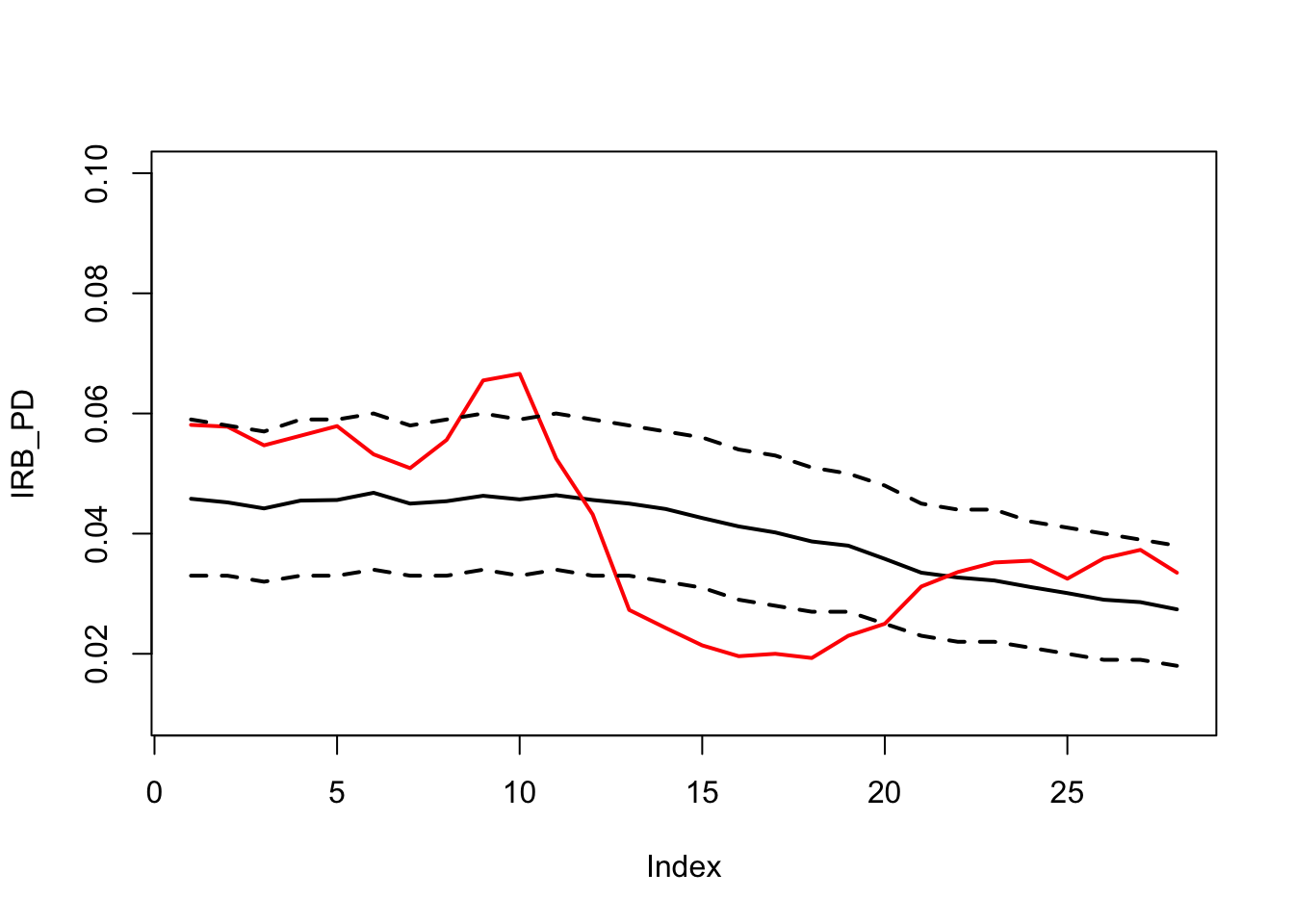

binomial_bounds(static_size=200)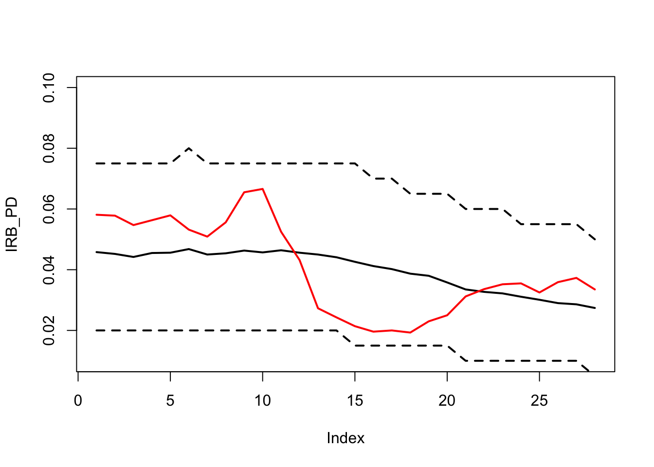

7. Estimate asset correlation \(\rho\)

The asset correlation \(\rho\) can be estimated from the default rate. Following the equation above:

\[ \begin{aligned} PD_{PiT} &= {P}(A_i(T)<L_i)\\ &= \Phi(\frac{\Phi^{-1}(PD_i^{*}) -\sqrt{\rho} \cdot Z}{\sqrt{1-\rho}}) \\ \end{aligned} \]

again, the \(PD_{i}^*\) is the \(PD_{TtC}\).

Then,

\[ \begin{aligned} \Phi^{-1}(PD_{PiT}) &= \frac{\Phi^{-1}(PD_i^{*}) -\sqrt{\rho} \cdot Z}{\sqrt{1-\rho}} \\ Var [\Phi^{-1}(PD_{PiT})]&= Var[\frac{\Phi^{-1}(PD_i^{*}) -\sqrt{\rho} \cdot Z}{\sqrt{1-\rho}}] \\ Var [\Phi^{-1}(PD_{PiT})] &= \frac{1}{1-\rho} Var[\Phi^{-1}(PD_i^{*})] + \frac{\rho}{1-\rho} \cdot 1 \\ Var [\Phi^{-1}(PD_{PiT})] &= \frac{\rho}{1-\rho} \\ Var [\Phi^{-1}(PD_{PiT})] - \rho Var [\Phi^{-1}(PD_{PiT})] &= \rho \\ \rho (1+ Var[\Phi^{-1}(PD_{PiT})]) &= Var [\Phi^{-1}(PD_{PiT})]\\ \rho &= \frac{Var [\Phi^{-1}(PD_{PiT})]}{1+Var [\Phi^{-1}(PD_{PiT})]} \\ \end{aligned} \] assuming the \(PD_{TtC}\) (or \(PD_i^{*}\)) is constant, then \(Var[\Phi^{-1}(PD_{TtC})]=0\)

If there are multiple ratings in the pool, then \(PD_{TtC}\) of the portfolio is not constant (portfolio changes over time). Therefore, \(\rho\) would need to be estimated by maximum likelihood in this case.

avg_IRB_PD <- c(0.0458, 0.0452, 0.0442, 0.0455, 0.0456, 0.0468, 0.045, 0.0454, 0.0463, 0.0457
                , 0.0464, 0.0456, 0.045,0.0441, 0.0426, 0.0412, 0.0402, 0.0387, 0.0380, 0.0358
                , 0.0335, 0.0327, 0.0322, 0.0311, 0.0301, 0.0290, 0.0286, 0.0274)
default_rate <- c(0.0581, 0.0578, 0.0547, 0.0563, 0.0579, 0.0532, 0.0509, 0.0556, 0.0655, 0.0666
                  , 0.0525, 0.0432, 0.0273, 0.0243, 0.0214, 0.0196, 0.02, 0.0193,0.0230, 0.0250
                  , 0.0312, 0.0336, 0.0352,0.0355, 0.0325, 0.0359, 0.0373, 0.0335)
empirical_q <- rank(default_rate)/(length(default_rate)+1)

Vasicek_PDF <- function(PiT, IRB, AC) {
  Vasicek_PDF <- sqrt((1-AC)/AC) * exp(0.5*(qnorm(PiT)^2 - ( ( sqrt(1-AC)*qnorm(PiT)-qnorm(IRB))/sqrt(AC))^2) )
}
Vasicek_CDF <- function(PiT, IRB, AC) {
  Vasicek_CDF <- (1-pnorm(-qnorm(PiT)*sqrt(1-AC)-qnorm(IRB)/sqrt(AC)) )
}
Vasicek_ICDF <- function(CI, IRB, AC) {
  Vasicek_ICDF <- pnorm( (qnorm(IRB)-sqrt(AC)*qnorm(1-CI)) /sqrt(1-AC) )
}
rho_candidate <- seq(0.01,0.05,0.0001)
calibration_process <- as.data.frame(matrix(NA, nrow=length(rho_candidate), ncol=2))
for(i in 1:length(rho_candidate)) {
  sum_loglikelihood <- sum(log(Vasicek_PDF(PiT = default_rate, IRB = avg_IRB_PD, rho_candidate[i])))
  calibration_process[i,1] <- rho_candidate[i]
  calibration_process[i,2] <- sum_loglikelihood 
}
rho <- calibration_process[which(calibration_process[,2]==max(calibration_process[,2])),1]
PiT_empirical_q <- Vasicek_ICDF(CI=empirical_q, IRB=avg_IRB_PD, AC=rho)
plot(avg_IRB_PD, type='l', ylim=c(0,0.1), ylab = "PD", xlab = "Period", lwd=2)
lines(default_rate, col='red', lwd=2)
lines(PiT_empirical_q, col='orange', lwd=2)
legend(x=16, y=0.1, c("IRB TtC PD", "Observed Default rate","PiT adjusted PD"),col=c("black","red","orange"),lty=c(1,1,1))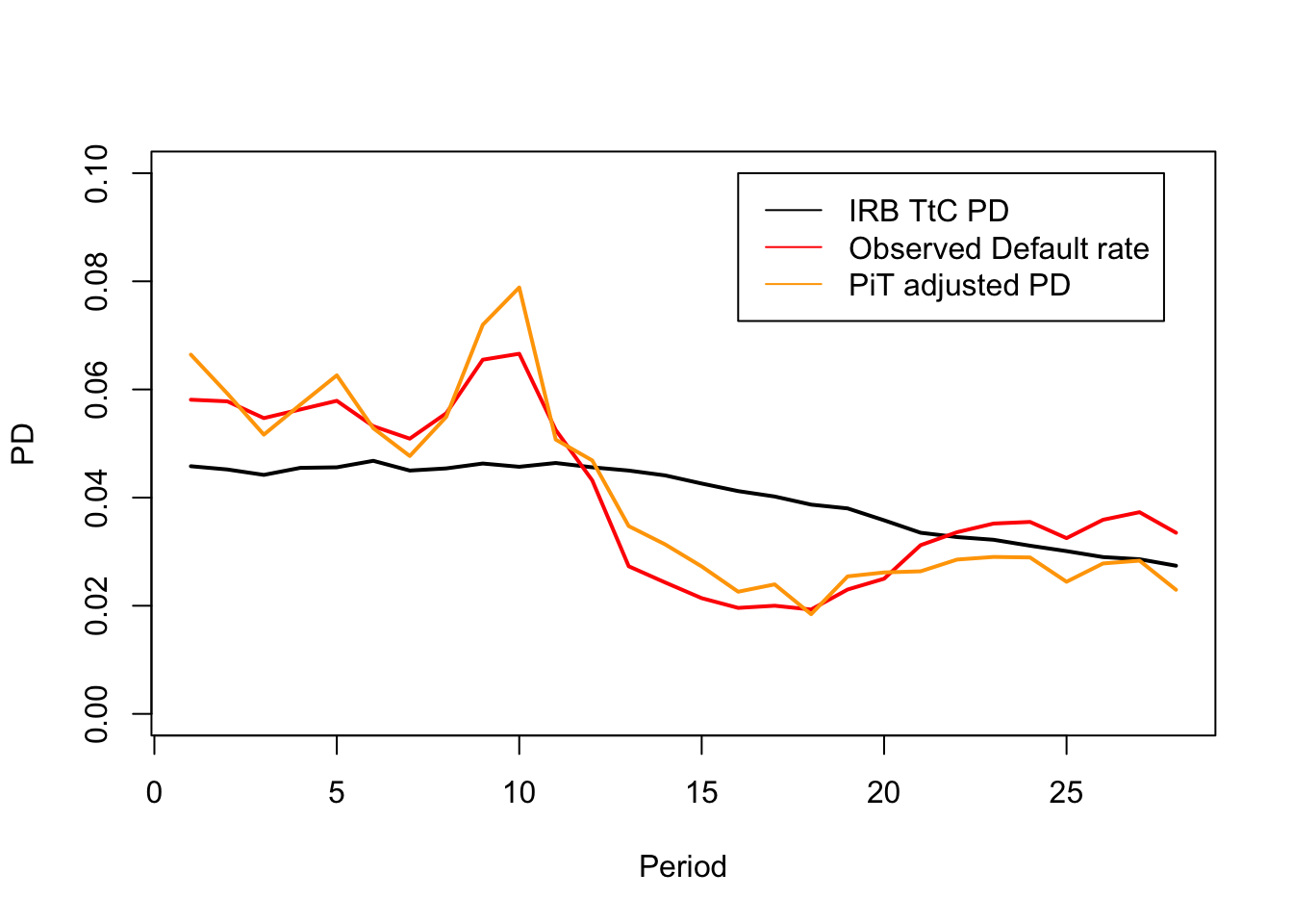

cat(paste0("The calibrated asset correlation is: ",rho*100,"% \n"))

## The calibrated asset correlation is: 2.61%

rho_p <- rho

8. Macro-economic model

Given the below formula derived in the previous section and the asset correlation \(\rho\) estimated by the approach above, now the only missing piece is the \(Z\) value, where \(Z \sim N(0,1)\).

\[ \begin{aligned} PD_{PiT} &= {P}(A_i(T)<L_i)\\ &= \Phi(\frac{\Phi^{-1}(PD_i^{*}) -\sqrt{\rho} \cdot Z}{\sqrt{1-\rho}}) \\ \end{aligned} \]

where \(PD_i^{*}\) is the TtC PD.

The \(Z\) value can be derived from the historical (same period as used for estimating \(\rho\)) macro-economic variables by following the below steps:

1. Derive the distribution parameters of the variables (Need to make assumptions for the variable first, e.g. S&P500 returns follow log normal distribution.)
2. Calculate the time series of parametric quantile for each point in the training period
3. Calculate the time series of standard normal \(Z\) value for each parametric quantile from above step
4. Calculate the time series of \(PiT_{PD}\) by using the formula above

The above steps can be repeated for multiple candidate variables, and the one with the highest predicting power for observed default rate would be chosen. Furthermore, a combination of multiple varialbes can also be used as the \(Z\) value and the weighted/cofficients be estimated by linear regression.

9. \(\rho\) and PiT distribution shape

The histagrams shows that as the \(\rho\) increase, the distribution becomes more flat tailed.

rho <- c(0.01,0.05,0.12)
ttc <- 0.05
n <- 2000
z <- rnorm(n, mean=0, sd=1)
pit <- matrix(nrow=n,ncol=3)
for(i in 1:n){
  pit[i,1] <- pnorm((qnorm(ttc)-sqrt(rho[1])*z[i])/sqrt(1-rho[1]),0,1)
  pit[i,2] <- pnorm((qnorm(ttc)-sqrt(rho[2])*z[i])/sqrt(1-rho[2]),0,1)
  pit[i,3] <- pnorm((qnorm(ttc)-sqrt(rho[3])*z[i])/sqrt(1-rho[3]),0,1)
}
par(mfrow=c(2,2))
hist(pit[,1], breaks=20,freq=FALSE, ylim=c(0,50), xlim=c(0,0.15), xlab='PiT PD', main = 'rho = 1%')
abline(v = ttc, col="red", lwd=2, lty=2)
hist(pit[,2], breaks=30, freq=FALSE, ylim=c(0,40), xlim=c(0,0.15), xlab='PiT PD', main = 'rho = 6%')
abline(v = ttc, col="red", lwd=2, lty=2)
hist(pit[,3], breaks=50, freq=FALSE, ylim=c(0,40), xlim=c(0,0.15), xlab='PiT PD', main = 'rho = 10%')
abline(v = ttc, col="red", lwd=2, lty=2)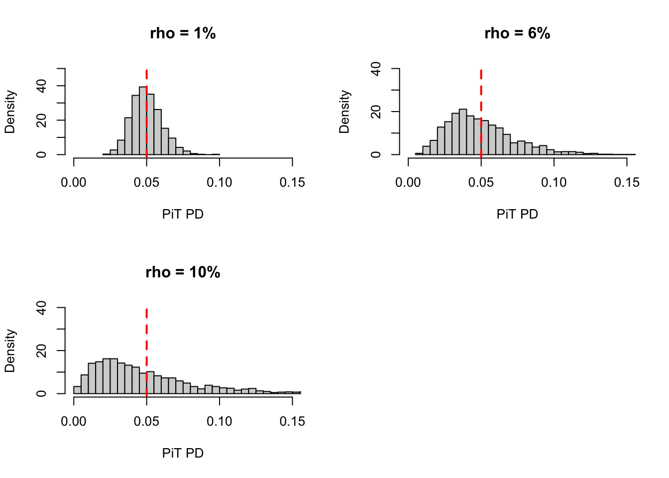

10. \(PD_{TtC}\) and variability

The histagram shows that the shape of PiT PD distributions are quite different given the same \(\rho\) but different \(PD_{TtC}\). Therefore, for different PD rating \(r_{i}\) (different \(PD_{TtC}\)), the \(\rho_{r_i}\) should be different to have the same shape.

rho <- 0.04
ttc <- c(0.01,0.06,0.24)
n <- 2000
z <- rnorm(n, mean=0, sd=1)
pit <- matrix(nrow=n,ncol=3)
for(i in 1:n){
  pit[i,1] <- pnorm((qnorm(ttc[1])-sqrt(rho)*z[i])/sqrt(1-rho),0,1)
  pit[i,2] <- pnorm((qnorm(ttc[2])-sqrt(rho)*z[i])/sqrt(1-rho),0,1)
  pit[i,3] <- pnorm((qnorm(ttc[3])-sqrt(rho)*z[i])/sqrt(1-rho),0,1)
}
par(mfrow=c(2,2))
hist(pit[,1], breaks=30, freq=FALSE, ylim=c(0,100), xlim=c(0,0.05), xlab='PiT PD', main = 'TtC = 1%')
abline(v = ttc[1], col="red", lwd=2, lty=2)
hist(pit[,2], breaks=30, freq=FALSE, ylim=c(0,30), xlim=c(0,0.25), xlab='PiT PD', main = 'TtC = 6%')
abline(v = ttc[2], col="red", lwd=2, lty=2)
hist(pit[,3], breaks=30, freq=FALSE, ylim=c(0,8), xlim=c(0,0.6), xlab='PiT PD', main = 'TtC = 24%')
abline(v = ttc[3], col="red", lwd=2, lty=2)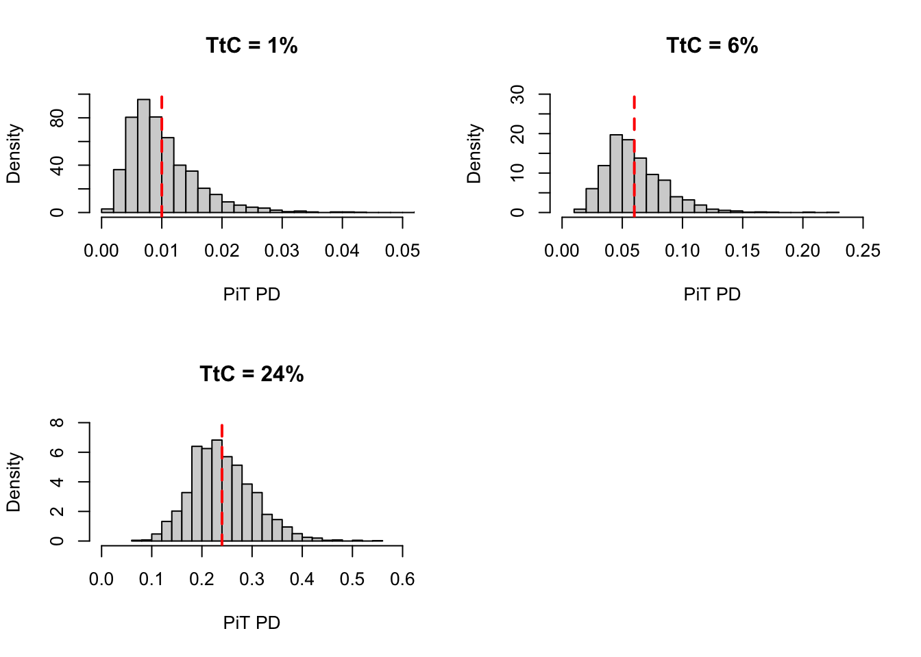

11. Asset correlation \(\rho\) per rating

The issue above presents when we estimate the asset correlation on portfolio level, but apply the same asset correlation to different ratings with different TtC PD.

rating_ts <- read.csv("~/Documents/GitHub/anpinHuang.github.io/ASRF_files/NumberPerRating_timeseries.csv")
IRB_TtC_PD <- c(0.001319,0.006152,0.01343,0.01812,0.03423,0.07932,0.09503,0.1488,0.2353)
PiT_PD_R <- matrix(0,nrow=nrow(rating_ts))
total_number <- rowSums(rating_ts)
for(r in 1:ncol(rating_ts)) {
  N_ratio <- rating_ts[,r]/total_number
  PiT_empirical_q_r <- Vasicek_ICDF(CI=empirical_q, IRB=IRB_TtC_PD[r], AC=rho_p)
  PiT_PD_R <- PiT_PD_R+N_ratio*PiT_empirical_q_r
}
plot(PiT_empirical_q, type='l', ylim=c(0,0.1), ylab = "PD", xlab = "Period", lwd=2)
points(PiT_empirical_q, col='black',pch=20)
lines(PiT_PD_R, col='orange', lwd=2)
points(PiT_PD_R, col='orange',pch=20)
legend(x=14, y=0.1, c("PiT PD", "PiT_PD_PL asset correlation"),col=c("black","orange"),lty=c(1,1), pch=c(20.20))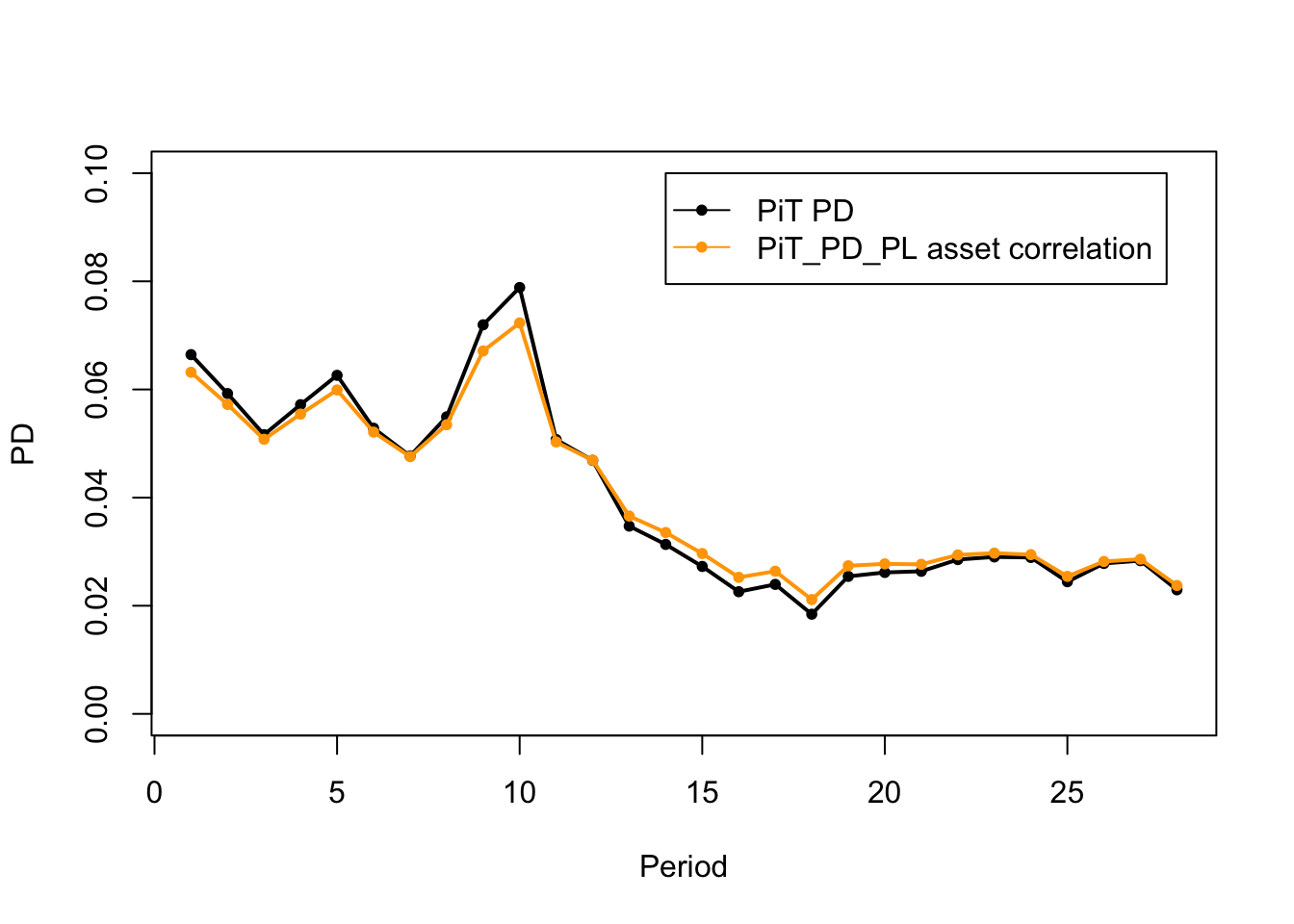

One solution is to estimate the asset correlation \(\rho\) individually for each rating. However, the data availability might be a problem for low default portfolio, especially for the high quality ratings where the default observation is even lower. Another approach to address this issue is to still estimate the \(\rho\) at the portfolio, but make the linear transformation adjustment for each rating.

\[\rho_r = \rho_{total} + (PD_{r}^{TtC}- \overline{DR_{total}}) \cdot \delta\]

The \(\delta\) parameter is determined by optimization:

\[ \underset{\delta}{\operatorname{argmin}} CV(PiT \ PD_{WARL}(t)) - CV(PiT \ PD_{PL}(t)) \]

where the coefficients of variance \(CV\) is the ratio of standard deviation divided by mean and

\[PiT \ PD_{WARL}(t) = \frac{\sum_{r=1}^{R}N_{r,t} \cdot F_{PD}^{-1}(PD_{r}^{TtC};\rho_{r};Q_t)}{\sum_{r=1}^{R} N_{r,t}} \]

\(N\) refers to number of observation, and \(Q\) refers to parametric quantile.

## calibrate delta
delta_candidate <- seq(-0.03,0.6,0.0001)
rho_R_I <- matrix(NA,nrow = length(delta_candidate), ncol=ncol(rating_ts))
avg_odr <- mean(PiT_empirical_q)
CV <- matrix(NA,nrow = length(delta_candidate), ncol=1)
total_number <- rowSums(rating_ts)
for(i in 1:length(delta_candidate)) {
  PiT_PD_R <- matrix(0,nrow=nrow(rating_ts))
  for(r in 1:ncol(rating_ts)) {
    rho_R_I[i,r] <- rho_p + (IRB_TtC_PD[r] - avg_odr)*delta_candidate[i]
    N_ratio <- rating_ts[,r]/total_number
    PiT_empirical_q_r <- Vasicek_ICDF(CI=empirical_q, IRB=IRB_TtC_PD[r], AC=rho_R_I[i,r])
    PiT_PD_R <- PiT_PD_R+N_ratio*PiT_empirical_q_r
  }
  CV[i,1] <- abs(sd(PiT_PD_R)/mean(PiT_PD_R) - sd(PiT_empirical_q)/mean(PiT_empirical_q))
}
delta <- delta_candidate[which(CV[,1]==min(CV[,1]))]
rho_R <- rho_R_I[which(CV[,1]==min(CV[,1])),]

## plot the PiT PD with AC per rating
PiT_PD_R <- matrix(0,nrow=nrow(rating_ts))
PiT_PD_r_adjusted <- matrix(0,nrow=nrow(rating_ts))
total_number <- rowSums(rating_ts)
for(r in 1:ncol(rating_ts)) {
  N_ratio <- rating_ts[,r]/total_number
  #PiT_empirical_q_r <- Vasicek_ICDF(CI=empirical_q, IRB=IRB_TtC_PD[r], AC=rho)
  #PiT_PD_R <- PiT_PD_R+N_ratio*PiT_empirical_q_r
  PiT_empirical_q_r_adj <- Vasicek_ICDF(CI=empirical_q, IRB=IRB_TtC_PD[r], AC=rho_R[r])
  PiT_PD_r_adjusted <- PiT_PD_r_adjusted+N_ratio*PiT_empirical_q_r_adj
}

plot(PiT_empirical_q, type='l', ylim=c(0,0.1), ylab = "PD", xlab = "Period", lwd=1)
points(PiT_empirical_q, col='black',pch=20)
lines(PiT_PD_r_adjusted, col='blue', lwd=1)
points(PiT_PD_r_adjusted, col='blue',pch=20)
legend(x=14, y=0.1, c("PiT PD","PiT PD rating asset correlation"),col=c("black","blue"),lty=c(1,1),pch=c(20,20))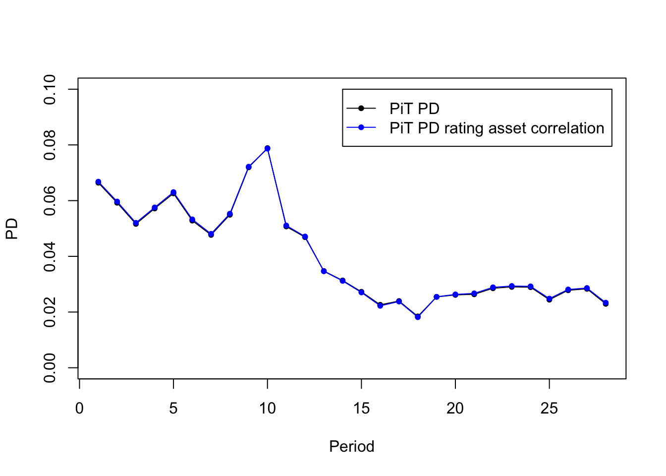

12. PiT non-default migration

With the TtC rating migration matrix, and PiT adjustment for default probability are established, the next step is the PiT adjustment for non-default rating migration.

\[MP^{PiT}_{r \to d} = F^{-1}_{PD}(MP^{TtC}_{r \to d};\rho_r;PiC)\]

• where \(r\) is the rating,

• \(d\) is the default state (rating) and

• \(MP^{PiT}_{r \to d}\) is the PiT migration probability from rating \(r\) to default \(d\), and is therefore also \(PD_{PiT}\).

• \(F^{-1}_{PD}\) is the inverse of Vasick distribution. recall that \(\Phi(\frac{\Phi^{-1}(PD_i^{*}) -\sqrt{\rho} \cdot Z}{\sqrt{1-\rho}})\)

• \(MP^{TtC}_{r \to d}\) refers to the \(PD_i^{*}\) in the previous equation

• \(PiC\) refers to the standard normal \(Z\) in the previous equation, but in here, it would be an actual number between 0 and 1 presribed by the economic scenario.

We can then derive the migration probability from \(r\) to one rating above default \(d-1\):

\[ \begin{aligned} MP^{PiT}_{r \to d-1} &= MP^{PiT}_{r \to \{d,d-1\}} - MP^{PiT}_{r \to d}\\ &= F^{-1}_{PD}(MP^{TtC}_{r \to \{d, d-1\}};\rho_r;PiC) - F^{-1}_{PD}(MP^{TtC}_{r \to d};\rho_r;PiC)\\ \end{aligned} \]

so on and so forth, we can derive the migration probability of \(r \to c\) where \(c\) is any non-default rating.

13. LGD for unresolved cases

• Includes all observed defaults. The CCR requires all observed default cases to be considered when estimating the LGD uner IRB approach.

  \(\to\) see (European Banking Association 2017) 6.5: “The CRR requirement that all observed defaults have to be taken into account applies to all LGD models under the IRB Approach, and hence no data exclusions are possible in the calculation of long-run average LGD. Furthermore, in the case of low-default portfolios the minimum requirements have to be met in order to receive permission to use the IRB Approach, and the CRR does not envisage any exemptions from these requirements for such portfolios.”

• Maximum recovery period. Institutions should estimate future recoveries only until a certain point in time (for IRB approach which requires conservatism). For IFRS 9 models, the maximum recovery period is incompliant as IFRS 9 models requires “best esimate” and does not allow conservatism.

  \(\to\) see (European Banking Association 2017): “Institutions should estimate future recoveries only until a certain point in time, i.e. the maximum length of the recovery process during which a sufficient number of recoveries were actually observed in similar cases.”

  \(\to\) see (European Banking Association 2017): “No further recoveries should be estimated beyond the maximum length of the recovery processes specified for the specific type of exposures.”

14. References

Basel Committee on Banking Supervision. 2005. An Explanatory Note on the Basel II IRB Risk Weight Functions. https://www.bis.org/bcbs/irbriskweight.pdf.

European Banking Association. 2017. Guidelines on PD and LGD Estimation (EBA-GL-2017-16).

Juulia Happonen. 2016. Theory Behind Regulatory Capital Formulae. https://aaltodoc.aalto.fi/bitstream/handle/123456789/22834/master_Happonen_Juulia_2016.pdf?sequence=1&isAllowed=y.